META TRADER 4 THREAD NOW ON KRESLIK.COM
Moderator: moderators
- TheRumpledOne
- rank: 10000+ posts
- Posts: 15570
- Joined: Sun May 14, 2006 9:31 pm
- Reputation: 3036
- Location: Oregon
- Real name: Avery T. Horton, Jr.
- Gender:
- Contact:
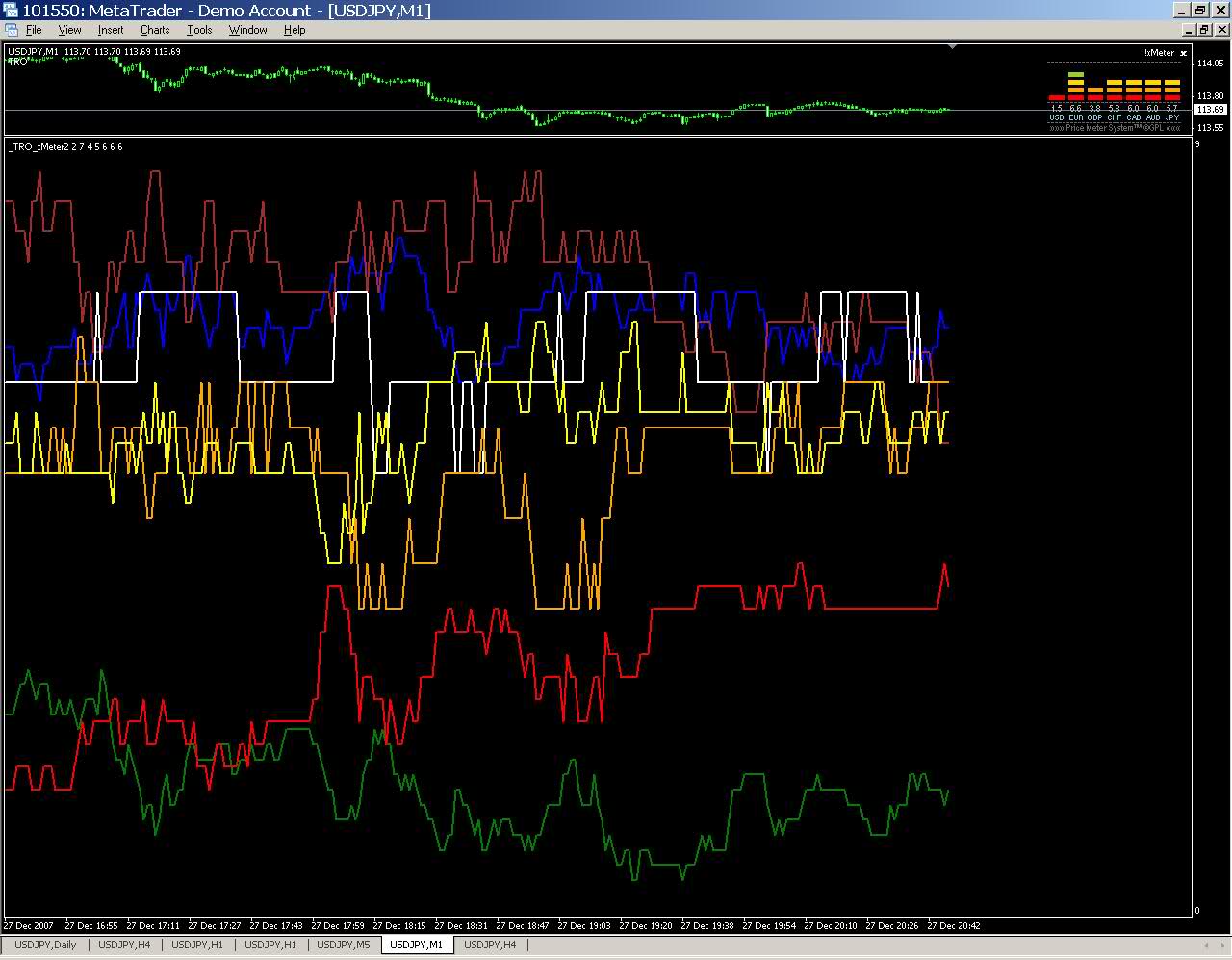
I turned the xMeter into a chart so you can see the history of the strength/weakness of the currencies.
Since this uses bid/ask info, when you load it up, it will NOT plot any history but will start from the load time. Just leave it running and the chart will fill out.
- Attachments
-
- TRO_xMeter.zip
- (7.34 KiB) Downloaded 327 times
Last edited by TheRumpledOne on Mon Apr 07, 2008 1:06 pm, edited 1 time in total.
IT'S NOT WHAT YOU TRADE, IT'S HOW YOU TRADE IT!
Please do NOT PM me with trading or coding questions, post them in a thread.
Please add www.kreslik.com to your ad blocker white list.
Thank you for your support.
- TheRumpledOne
- rank: 10000+ posts
- Posts: 15570
- Joined: Sun May 14, 2006 9:31 pm
- Reputation: 3036
- Location: Oregon
- Real name: Avery T. Horton, Jr.
- Gender:
- Contact:
More MT4 code and updates.
- Attachments
-
- MT4_2007Dec27.zip
- (246.41 KiB) Downloaded 375 times
IT'S NOT WHAT YOU TRADE, IT'S HOW YOU TRADE IT!
Please do NOT PM me with trading or coding questions, post them in a thread.
- TheRumpledOne
- rank: 10000+ posts
- Posts: 15570
- Joined: Sun May 14, 2006 9:31 pm
- Reputation: 3036
- Location: Oregon
- Real name: Avery T. Horton, Jr.
- Gender:
- Contact:
MACD meter.
- Attachments
-
- tro_macd.zip
- (24.67 KiB) Downloaded 316 times
IT'S NOT WHAT YOU TRADE, IT'S HOW YOU TRADE IT!
Please do NOT PM me with trading or coding questions, post them in a thread.
- TheRumpledOne
- rank: 10000+ posts
- Posts: 15570
- Joined: Sun May 14, 2006 9:31 pm
- Reputation: 3036
- Location: Oregon
- Real name: Avery T. Horton, Jr.
- Gender:
- Contact:
More MT4 code
- Attachments
-
- MT4_2007Dec28.zip
- (209.39 KiB) Downloaded 353 times
IT'S NOT WHAT YOU TRADE, IT'S HOW YOU TRADE IT!
Please do NOT PM me with trading or coding questions, post them in a thread.
Please add www.kreslik.com to your ad blocker white list.
Thank you for your support.
- TheRumpledOne
- rank: 10000+ posts
- Posts: 15570
- Joined: Sun May 14, 2006 9:31 pm
- Reputation: 3036
- Location: Oregon
- Real name: Avery T. Horton, Jr.
- Gender:
- Contact:
I added the RSI METER and improved/fixed the MA and MACD meters.
- Attachments
-
- TRO_Meters.zip
- (78.14 KiB) Downloaded 389 times
IT'S NOT WHAT YOU TRADE, IT'S HOW YOU TRADE IT!
Please do NOT PM me with trading or coding questions, post them in a thread.
- TheRumpledOne
- rank: 10000+ posts
- Posts: 15570
- Joined: Sun May 14, 2006 9:31 pm
- Reputation: 3036
- Location: Oregon
- Real name: Avery T. Horton, Jr.
- Gender:
- Contact:
-
- rank: <50 posts
- Posts: 2
- Joined: Mon Dec 24, 2007 9:10 pm
- Reputation: 0
- Gender:
TRO,
Please can you convert this ELD to MetaTrader?
I am no longer with TradeStation so cannot show you a snapshot of the indicator.
Thanks much for your help.
Please can you convert this ELD to MetaTrader?
I am no longer with TradeStation so cannot show you a snapshot of the indicator.
Code: Select all
{
XCAP_iPolyCycle
Author: Paul A. Griffin
January 16, 2007
Extrema Capital, 2007
Introduction:
This is an example of what can be done by combining Legendre polynomials and
analytic signals. I get a way of determining a smooth period and
relative adaptive strength indicator without adding time lag.
This indicator displays the following:
a. The Least Squares fit of a polynomial to a DC subtracted time series - a best fit to a cycle.
b. The normalized analytic signal of the cycle (signal and quadrature).
c. The Phase shift of the analytic signal per bar.
d. The Period and HalfPeriod lengths, in bars of the current cycle.
e. A relative strength indicator of the time series over the cycle length. That is, adaptive
relative strength over the cycle length.
The Relative Strength Indicator, is adaptive to the time series, and it can be smoothed by increasing the length of
decreasing the number of degrees of freedom.
Other adaptive indicators based upon the period and can be similarly constructed.
There is some new math here, so I have broken the story up into 5 Parts:
Part 1:
Any time series can be decomposed into a orthogonal set of polynomials [1,2,3].
This is just math and here are some good references:
[1] http://en.wikipedia.org/wiki/Legendre_polynomials
[2] https://www.tradestation.com/Discussions/Topic.aspx?Topic_ID=59250
[3] Peter Seffen, "On Digital Smoothing Filters: A Brief Review of Closed Form Solutions and Two New Filter Approaches",
Circuits Systems Signal Process, Vol. 5, No 2, 1986
I gave some thought to what should be done with ths and came to the conclusion that they can be used for basic smoothing
of time series. For the analysis below, I decompose a time series into a low number of
degrees of freedom and discard the zero mode to introduce smoothing.
That is:
time series => c_1 t + c_2 t^2 ... c_Max t^Max
This is the cycle. By construction, the cycle does not have a zero mode and more physically, I am defining the
"Trend" to be the zero mode.
The data for the cycle and the fit of the cycle can be viewed by setting
ShowDataAndFit = TRUE;
There, you will see the fit of the last bar as well as the time series of the leading edge of the fits. If you don't
know what I mean by the "leading edge", please see some of the postings in [2]. The leading edges are in grayscale,
and the fit of the last bar is in color.
I have choosen Length = 17 and Degree = 4 as the default. I am simply making sure by eye that the fit is reasonably good and
degree 4 is the lowest polynomial that can represent a sine-like wave, and 17 is the smallest length that lets me calculate
the Phase Shift (Part 3 below) using the Hilbert Transform of width=7 (Part 2 below).
Depending upon the fit you make, you will capture different cycles in the data. A fit that is too "smooth" will
not see the smaller cycles, and a fit that is too "choppy" will not see the longer ones. The idea is to use the fit
to try to suppress the smaller noise cycles while keeping larger signal cycles.
Part 2:
Every time series has an Analytic Signal, defined by applying the Hilbert Transform to it. You can think of the
original time series as amplitude * cosine(theta) and the transformed series, called the quadrature, can be thought of as
amplitude * sine(theta). By taking the ratio, you can get the angle theta, and this is exactly what was done by
John Ehlers in [4]. It lets you get a frequency out of the time series under consideration.
[4] http://www.amazon.com/Rocket-Science-Traders-Processing-Applications/dp/0471405671
It helps to have more references to understand this. There is a nice article in Wikipedia[5] on it.
Read the part about the discrete Hilbert Transform:
[5] http://www.answers.com/topic/hilbert-transform
Also, Answers.com has good information on the Hilbert Transform and links to other concepts:
[6] http://www.answers.com/topic/hilbert-transform
If you really want to understand how to go from continuous to discrete, look up this article
written by Richard Lyons:
[7] www.dspguru.com/info/tutor/QuadSignals.pdf
In the indicator below, I am calculating the normalized analytic signal,
which can be written as:
s + i h where i is the imagary number, and s^2 + h^2 = 1;
s= signal = cosine(theta)
h = hilbert transformed signal = quadrature = sine(theta)
The angle is therefore given by theta = arctan(h/s);
The analytic signal leading edge and the fit of the last bar of the cycle can be viewed by setting
ShowAnalyticSignal = TRUE;
The leading edges are in grayscale fit to the last bar is in color. Light (yellow) is the
s term, and Dark (orange) is the quadrature (hilbert transform). Note that for every bar,
s^2 + h^2 = 1 , by construction.
I am using a width = 7 Hilbert transform, just like Ehlers. (But you can adjust it if you want.) This transform has a
7 bar lag. I have put the lag into the plot statements, so the cycle info should be quite good at displaying minima
and maxima (extrema).
Part 3:
The Phase shift is the amount of phase change from bar to bar.
It is a discrete unitary transformation that takes s[1] + i h[1] to s + i h
explicitly, T = (s+ih)*(s[1]-ih[1]) , since s[1]*s[1] + h[1]*h[1] = 1.
writing it out, we find that T = T1 + iT2
where T1 = s*s[1] + h*h[1] and T2 = s*h[1]-h*s[1]
and the phase shift is given by PhaseShift = arctan(T2/T1);
Alas, I have no reference for this, all I doing is finding the rotation what takes the analytic signal
at bar [1] to the analytic signal at bar [0]. T is the transfer matrix.
Of interest is the PhaseShift from the closest two bars to the present, given by the
bar [7] and bar [8] since I am using a width=7 Hilbert transform, bar [7] is the earliest bar with an
analytic signal.
I store the phase shift from bar [7] to bar [8] as a timeseries called PhaseShift. It basically gives
you the (7-bar delayed) leading edge the amount of phase angle change in the series.
You can see it by setting
ShowPhaseShift=TRUE
The green points are positve phase shifts and red points are negative pahse shifts.
On most charts, I have looked at, the indicator is mostly green, but occationally, the stock
"retrogrades" and red appears. This happens when the cycle is "broken" and the cycle length starts to
expand as a trend occurs.
Part 4:
The Period:
The Period is the number of bars required to generate a sum of
PhaseShifts equal to 360 degrees.
The halfperiod is the number of bars required to generate a sum of phase shifts
equal to 180 degrees. It is usually not equal to 1/2 of the period.
You can see the Period and Halfperiod by setting
ShowPeriod=TRUE
The code is very simple here:
Value1=0;
Value2=0;
while Value1 < barnumber and AbsValue(Value2) < 360 begin
Value2 = Value2 + PhaseShift[Value1];
Value1 = Value1 + 1;
end;
Period = Value1;
The period is sensitive to the input length and degree values but not overly so. Any insight
on this would be appreciated.
Part 5:
The Relative Stength indicator:
The Relative Strength is just the current value of the series minus the minimum over the last cycle
divided by the maximum - minimum over the last cycle, normalized between +1 and -1.
RelativeStrength = -1 + 2*(Series-Min)/(Max-Min);
It therefore tells you where the current bar is relative to the cycle. If you want to smooth the indicator, then
extend the period and/or reduce the polynomial degree.
In code:
NewLength = floor(Period + HilbertWidth+1);
Max = highest(Series,NewLength);
Min = lowest(Series,NewLength);
if Max>Min then
Note that the variable NewLength includes the lag that comes from the hilbert transform,
(HilbertWidth=7 by default).
Conclusion:
This is an example of what can be done by combining Legendre polynomials and
analytic signals to determine a smooth period without adding time lag.
}
Inputs:
Series((h+l)/2),
Length(17), // Length = 2*Width+1, the minimum is 17 bars
Degree(4), // 0 <= Degree <= 2*Width+1, default is 4, 4 DOF for 17 bars
ShowDataAndFit(FALSE), //Shows data and fit of the data last bar only
ShowAnalyticSignal(FALSE), //Shows the signal between the
ShowPhaseShift(FALSE), //Shows the PhaseShift for the last bar
ShowPeriod(FALSE), //Shows the number of bars required to Phase Shift a half and a full period
ShowRelativeStrength(TRUE); //Show the relative strengh of the current bar w.r.t. a full period (+ calculation lag).
Variables:
HilbertWidth(7), // Must be an odd number. 1,3,5,7,9, ... less than or equal to Width = floor(Length-1)/2)
pi(3.141592653589793), //close enough
Width(floor((Length-1)/2)); //
Variables:
DC(0),
EarliestWidth(0),
LeadingCycleEdge(0),
LeadingSignalEdge(0),
LeadingHilbertEdge(0),
p(0),j(0),k(0),
DataSize(2*Width+1),
T1(0),T2(0),//TransferMatrix
PhaseShift(0),
HalfPeriod(0),Period(0),
Max(0),Min(0),
RelativeStrength(0);
Arrays:
Polynomial[](0),
Coefficient[](0),
Cycle[](0),
Signal[](0),
Hilbert[](0),
HilbertTransform[](0),
SignalTransform[](0);
if barnumber = 1 then begin
//Allocate memory for the arrays. Polynomial is a 2D array
Array_SetMaxIndex(Polynomial, DataSize*(Degree+1)+1);
Array_SetMaxIndex(Coefficient, Degree+1);
Array_SetMaxIndex(Cycle, DataSize);
Array_SetMaxIndex(Signal, DataSize);
Array_SetMaxIndex(Hilbert, DataSize);
//We are going to make the analytic signal of the time series with the transforms below:
Array_SetMaxIndex(HilbertTransform, 2*HilbertWidth+1);
Array_SetMaxIndex(SignalTransform,2*HilbertWidth+1);
//Create the Dicrete Hilbert Transform Filter, normalized to a step function (the last being my idea)
for k = -HilbertWidth to HilbertWidth begin
if mod(k,2) = 0 then HilbertTransform[HilbertWidth+k] = 0 else HilbertTransform[HilbertWidth+k] = 2/(pi*k);
if k = 0 then SignalTransform[HilbertWidth+k] = 1 else SignalTransform[HilbertWidth+k] = 0;
end;
end;
//Determine earliest bar required for analysis and plotting to save time
if LastBarOnChart = TRUE then EarliestWidth = - Width else EarliestWidth = Width - 2*HilbertWidth-1;
/////////////////////////////////////////////////////////////////////
// Decompose data into the polynomial set and determine the overlap coefficients:
//
// This is the basic decomposition step
for p = 0 to Degree begin
Coefficient[p] = 0;
for j = -Width to + Width begin
Coefficient[p]= Coefficient[p] + Polynomial[p*DataSize+Width+j]*Series[Width-j];
end;
end;
//
/////////////////////////////////////////////////////////////////////
// Remap to the Cycle to create the Cycle time series, remove the 0 mode, and the modes higher than Degree.
//
DC = Coefficient[0]*Polynomial[Width+Width];
for j = EarliestWidth to Width begin
Cycle[Width+j] = 0;
for p = 1 to Degree begin //p=0 removed
Cycle[Width+j] = Cycle[Width+j] + Coefficient[p]*Polynomial[p*DataSize+Width+j];
end;
end;
//
////////////////////////////////////////////////////////////////////////
/////////////////////////////////////////////////////////////////////////
// Signal and Hilbert Of the Cycle: Create the Analytic time series
//
for j = EarliestWidth + HilbertWidth to Width - HilbertWidth begin
Signal[Width+j]=0;
Hilbert[Width+j] = 0;
//Execute the Transforms
for k = -HilbertWidth to HilbertWidth begin
Hilbert[Width+j] = Hilbert[Width+j] + HilbertTransform[HilbertWidth+k] * Cycle[Width+j+k];
Signal[Width+j] = Signal[Width+j] + SignalTransform[HilbertWidth+k] * Cycle[Width+j+k];
end;
//The normalized with respect to the amplitude
Value1 = Power(Signal[Width+j],2) + Power(Hilbert[Width+j],2);
if Value1>0 then begin
Value1 = Power(Value1,-0.5);
Signal[Width+j]= Value1 * Signal[Width+j];
Hilbert[Width+j]= Value1 * Hilbert[Width+j];
end;
end;
//
//////////////////////////////////////////////////////////////////////////
//////////////////////////////////////////////////////////////////////////
// The Phase Shift of the leading edge bar change, by Paul Griffin
T1 = Signal[2*Width-HilbertWidth]*Signal[2*Width-HilbertWidth-1] +
+ Hilbert[2*Width-HilbertWidth]*Hilbert[2*Width-HilbertWidth-1];
T2 = -Hilbert[2*Width-HilbertWidth]*Signal[2*Width-HilbertWidth-1]
+ Signal[2*Width-HilbertWidth]*Hilbert[2*Width-HilbertWidth-1];
If T1 <> 0 then PhaseShift = Arctangent(T2 / T1);
//
//////////////////////////////////////////////////////////////////////
//////////////////////////////////////////////////////////////////////
// Add phase shifts to determine the period and halfperiod, by Paul Griffin
//period
Value1=0;
Value2=0;
while Value1 < barnumber and AbsValue(Value2) < 360 begin
Value2 = Value2 + PhaseShift[Value1];
Value1 = Value1 + 1;
end;
Period = Value1;
//halfperiod
Value1=0;
Value2=0;
while Value1 < barnumber and AbsValue(Value2) < 180 begin
Value2 = Value2 + PhaseShift[Value1];
Value1 = Value1 + 1;
end;
HalfPeriod = Value1;
//Store the leading edges for display purposes
LeadingSignalEdge = Signal[Width+Width - HilbertWidth];
LeadingHilbertEdge = Hilbert[Width+Width - HilbertWidth];
LeadingCycleEdge = Cycle[Width+Width];
//////////////////////////////////////////////////////////////////
// The Relative Strength, this is the easy part
Value1 = floor(Period + HilbertWidth+1);
Max = highest(Series,Value1);
Min = lowest(Series,Value1);
if Max>Min then RelativeStrength = -1 + 2*(Series-Min)/(Max-Min);
//
//////////////////////////////////////////////////////////////////
//////////////////////////////////////////////////////////////////
//
// Plotting routines
if LastBarOnChart = TRUE and ShowDataAndFit = TRUE then begin
for j = EarliestWidth to Width begin
plot1[Width-j](Series[Width-j]-DC,"Data",cyan);
plot2[Width-j](Cycle[Width+j],"Cycle",blue);
end;
end;
if barnumber>1 and ShowDataAndFit = TRUE then begin
plot3(Series-DC,"LeadingData",lightgray);
plot4(LeadingCycleEdge,"LeadingCycle",white);
end;
if LastBarOnChart = TRUE and ShowAnalyticSignal = TRUE then begin
for j = -Width + HilbertWidth to Width - HilbertWidth begin
plot5[Width-j](Signal[Width+j],"Signal",yellow);
plot6[Width-j](Hilbert[Width+j],"Quadrature",RGB(255,128,0));
end;
end;
if barnumber>1 and ShowAnalyticSignal = TRUE then begin
Plot7[HilbertWidth](LeadingSignalEdge,"SignalEdge",lightgray);
Plot8[HilbertWidth](LeadingHilbertEdge,"QuadEdge",darkgray);
end;
if barnumber>1 and ShowPhaseShift = TRUE then begin
if T2>0 then Plot9[HilbertWidth](PhaseShift,"PhaseShift",green);
if T2<0 then Plot9[HilbertWidth](PhaseShift,"PhaseShift",red);
end;
if barnumber>1 and ShowPeriod=TRUE then begin
Plot10[HilbertWidth](Period,"Period",yellow);
Plot11[HilbertWidth](HalfPeriod,"HalfPeriod",RGB(255,128,0));
end;
if barnumber>1 and ShowRelativeStrength=TRUE then begin
plot12(RelativeStrength,"RelStrength",white);
end;
Plot99(0,"0",white);
//
///////////////////////////////////////////////////////////////
///////////////////////////////////////////////////////////////
//
// Create the Orthoginal Legendre Polynomials during the first bar
//
////////////////////////////////////////////////////////////////
if barnumber = 1 then begin
//The first polynomial is a constant, easy to create
for j = - Width to + Width begin
Polynomial[0*DataSize + Width+j] = 1;
end;
//The second polynomial is a line
if Degree>=1 then begin
for j = -Width to +Width begin
Polynomial[1*DataSize + Width+j] = j;
end;
end;
//We use the discrete Legendre polynomial recurrence relations to create the rest
if Degree > 1 then begin
for p = 1 to Degree - 1 begin // create the polynomial for degree p+1
for j = -Width to Width begin // sum over the interval
Value1 = j*(2*p+1)/(p+1); //discrete Legendre polynomial solution
Value2 = - (p/(p+1))*(2*Width+1+p)*(2*Width+1-p)/4; //discrete Legendre polynomial solution
Polynomial[(p+1)*DataSize+Width+j] //The recurrence relation
= Value1 * Polynomial[p*DataSize+Width+j] + Value2 * Polynomial[(p-1)*DataSize+Width+j];
end;
end;
end;
//Now we have to normalize each polynomial, so that the sum of the square of the polynomial
//over the interval is 1. Instead of doing the calculation however, we apply the pre-determined answer[4]:
for p = 0 to Degree begin
Value1 = Power(2,-2*p)/(2*p+1);
for j = -p to p begin Value1 = Value1 * (2*Width+1+j); end;
if Value1 > 0 then Value1 = 1/squareroot(Value1); //this is the normalization coefficient
for j = -Width to +Width begin
Polynomial[p*DataSize+Width+j] = Value1 * Polynomial[p*DataSize+Width+j];
end;
end;
//Done! We now have a orthogonal normalized set of polynomials
end;
Thanks much for your help.
- TheRumpledOne
- rank: 10000+ posts
- Posts: 15570
- Joined: Sun May 14, 2006 9:31 pm
- Reputation: 3036
- Location: Oregon
- Real name: Avery T. Horton, Jr.
- Gender:
- Contact:
NO.
I am not programming other people's code into MT4.
I am only programming the tools necessary for my style of trading.
I am sure you can find something like the code you want. There are THOUSANDS of free MT4 programs on the net.
I am not programming other people's code into MT4.
I am only programming the tools necessary for my style of trading.
I am sure you can find something like the code you want. There are THOUSANDS of free MT4 programs on the net.
IT'S NOT WHAT YOU TRADE, IT'S HOW YOU TRADE IT!
Please do NOT PM me with trading or coding questions, post them in a thread.
Please add www.kreslik.com to your ad blocker white list.
Thank you for your support.